The Species Construction Manual

(Draft version. Further description of the graphical contents will follow soon.)

Contents of this page

	Introduction
	Preconsiderations
	Parametrization of plant structure
	- Organ parametrization
	- - Leaf parametrization
	- - Stem and internode parametrization
	- - Flower parametrization
	- - Clonal growth organ parametrization
	- - Roots parametrization
	- - - Method for species-specific root traits retrieval
	- Parametrization of partitioning
	- Parametrization of ramet growth
	- Parametrization of branching
	Parametrization of plant function
	- Parametrization of organ function
	- - Mass- and energy exchange parametrization
	- - - Leaf parametrization
	- - - Internode parametrization
	- - - Root and CGO parametrization
	- - Parametrization of organ aging
	- - Parametrization of C-/N-storage
	Outline: Closing the plant life cycle
	Scaling up from the organ to the canopy level
	- Atmospheric environment at reference height
	- Atmospheric environment above the canopy
	- Atmospheric environment within the canopy
	- - Radiation interception model
	- - Turbulent transfer model

Top_________________________Next

Introduction

	This section deals with the ecological issues of model building. It details the general methodology for species construction from databases that has been developed within UIBM using Arrhenatherum elatius as template species. Hence, this section does represent a "Species Construction Manual".
	Again, once a template species is successfully constructed from databases, more species are to be constructed with ease. This is the basic idea that makes UIBM a biodiversity model.
	Therefore, the assessment of which Arrhenatherum elatius traits could be derived from databases is a major purpose here. Throughout this section such traits are marked in the figures in green with a "barrel" symbolizing a database source.
	In contrast, traits being derived merely from the literature are marked in red with a "Non-barrel" icon.
	Moreover, in this section the main assumptions underlying UIBM are specified and marked in lila with a thought bubble in the figures.
	Figures are interspersed by discussions of the parametrization aspects at appropriate places. When parametrization of the template species had to rely on literature sources suggestions of database improvements are made or implications for future species parametrizations are addressed.
	A general discussion of species parametrization from databases completes the section.

Top_________________________Next

Preconsiderations

	Cardinal model characteristics, such as spatial and temporal scale, were defined in an early stage of the UIBM development.
	UIBM's spatial scale is oriented towards the relevé size of the phytosociological method to real-world vegetation sampling and classification (Barbour et al. 1999). Within the method invented by Braun-Blanquet the size of a relevé ranges slightly above that of the minimal area, which holds a certain large fraction, usually 95%,of the species number the vegetation type contains (Barbour et al. 1999). The relevé size, in principle, ensures that a representative fraction of the community in question is sampled.
	Recently, Chytrý & Otýpková have suggested 16m² as standard relevé size for most European grassland, heathland and other herbaceous or low-scrub vegetation types (Chytrý & Otýpková 2003). Hence, 16 m² is also the spatial scale I chose for UIBM's virtual vegetation survey plots.
	Due to a lack of experience with comparing real-world data with model results so far only preliminary considerations with respect to temporal scale can be given here.
	The minimum duration given in Figure 24, i.e. five years, is guided by the following reasoning: The clonal growth organ (CGO) of Arrhenatherum elatius possesses a lifespan of more than two years. Thus, it will likewise take Arrhenatherum more than two years until the clonal plant breaks apart for the first time to form two ramet networks. Even more time is likely needed to reach a steady state of CGO dieback and formation within a closed canopy. To enable this kind of established canopy to develop I set the minimum duration to 5 years, though.
	With 50 years the upper limit to the temporal scale was chosen to allow for a significant biodiversity response to occur, but to not let model results vary without bounds depending on the selected environmental scenario.
	Since UIBM with its functional basis relies on a canopy gas exchange model simulation time proceeds at an interval of one or two hours, respectively.
	A definition of the individual concept as it is used in the Universal Individual-Based Model shall also be given in this section.
	In a forest growth model the individual is easy to identify and well defined: The individual is a single tree with its rooting system, its trunk and its crown. Unlike, in herbaceous systems and in grassland systems, in particular, the individual is more difficult to identify in the field. Certainly, in these systems the ramet network is the individual. The ramet network is a set of ramets interconnected and, hence, synchronized by their common clonal growth organ(s). However,in UIBM the ramet is considered to act almost autonomously and behaves much like an individual, though. One exception with respect to ramet autonomy is made: The carbon storage of the clonal growth organs as well as the nitrogen storage is shared among the ramets belonging to a ramet network. In case the C/N-ratio in the resources a ramet acquires leaves the allowable range, e.g. when a ramet does not acquire sufficient carbon, the necessary storage compounds are made available to that ramet by the ramet network. Basically, this all-or-nothing behavior is UIBM's first simplifying assumption.
	Main sources of trait information are contained in the table of Figure 24. The left column shows the databases together with their abbreviations which are used in the figures to come. In the right column you can find major information sources other than databases, i.e. literature sources, which are referred to in the following paragraphs by their identification number.

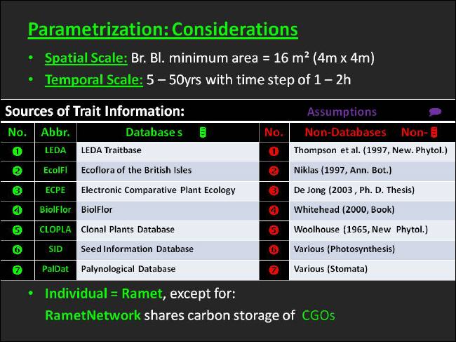
Fig. 24: Preconsiderations to the parametrization

Top_________________________Next

Parametrization of plant structure

Organ parametrization

	Furnishing UIBM with a functional basis puts certain requirements on the organ traits to be included in the model.
	The organ gas exchange, albeit photosynthesis or respiration, depends on organ nitrogen concentration and, thus. N-concentrations have to be inserted.
	The leaf is the plant organ which is most frequently studied, and information about leaf [N] is most readily available for many species, though. The situation, however, is inferior for the remaining plant organs. Therefore, the inference of organ N-concentrations from leaf [N] using organ nitrogen relationships seemed most promising in the context of UIBM.
	The relationships we use in UIBM were taken from verbal descriptions made by Whitehead (2001) in his comprehensive book "Nutrient Elements in Grassland".
	On this basis we presume that internode [N] is one third and fine root [N] is half of leaf N-concentration.
	The assignment of clonal growth organ [N] depends on the CGO-type. Since the CGO type of Arrhenatherum elatius, i.e. CGO type 10 (compare CLOPLA), originates from the stem, we assigned the CGO [N] to the internode N-concentration in this case.
	The procedure outlined here is graphically summarized in Figure 25. Since the procedure is based on literature sources rather than databases it is marked with the "Non-Barrel" icon in red and a reference to 2 = Whitehead (2001) is given in Figure 25.

Top_________________________Next

Leaf parametrization

	Nowadays, the GLOPNET database of Wright et al. (2004) is most likely the primary source for mass- and area-based leaf traits data.
	Unfortunately, neither Wright et al. (2004) nor any of the publications they quote as sources for European herbaceous plant species data in the supplementary information to their article (Diemer, Körner & Prock 1992, Cornelissen & Thompson 1997, Poorter & De Jong 1999, cited therein) provide data in the form required by UIBM, i.e. trait minima and trait maxima representative for the range of field conditions in the region.
	Although the contributors to GLOPNET may also provide data on leaf trait variation on request, we preferred to obtain leaf [N] minima/maxima for Arrhenatherum elatius from a UK field survey taken by Thompson et al. (1997). In their survey Thompson et al. determined mineral nutrient concentrations in leaves of 83 mostly herbaceous species sampled in Central England. As with most other databases this survey included also leaf phosphorus concentrations, but many more nutrients have been measured within this study.
	Leaf structural attributes, in general, depend on the composition of mineral nutrients in the leaf (Baker et al. 1985).
	Since nitrogen limitation to plant growth seems to be most widespread in nature (Vitousek & Howarth 1991), nitrogen dependency of leaf structure is accounted for in UIBM. In contrast, the influence of phosphorus on leaf structure has been neglected so far, because P-limitation is less prevalent (Vitousek & Howarth 1991). Nevertheless, at a later stage parametrization of the P-dependence from the data and its implementation via a subtle Liebig minimum law will be straightforward.
	It is well known, however, that leaf size increases with foliar N-concentration (Baker et al. 1985, Mengel & Kirkby 2001, Pea & Morot-Gaudry 2001). Stuart Chapin III (1980), although presenting a more differentiated view on this subject, points out that leaf size of forage grasses, in particular, is highly responsive to nutritional status. Thus, we associated the smallest leaf size in terms of leaf-mass and leaf-area contained in the LEDA traitbase with the minimum leaf [N], and vice versa.
	According to regional field guides the length of Arrhenatherum elatius leaves varies between 10 and 40 cm. Based on the same sources leaf width ranges from 0.4 to 1.0 cm. Assuming triangular leaf shapes the dimensional boundaries agreed well with those of leaf area. Nonetheless, I preferred to rely on the leaf area records from the LEDA traitbase and derive leaf dimensions from computed length:width ratios, i.e. 25 for minimum leaf [N] and 40 for maximum leaf [N], respectively. In the context of leaf dimensions field guides are considered a first-class source of information, comparable to databases, since it is supposed that data is available for all Central-European species from the guides.
	Scleromorphism has been reported as a common symptom of N-deficiency (compare Larcher 2003, Table 3.6, page 201). As Stuart Chapin III (1980) states low tissue concentrations, which are the norm for species growing on infertile soils, are associated with more structural tissue (often sclerophyllous leaves). More specifically, many authors have noted that high specific leaf area (SLA = leaf area per leaf mass) is a characteristic of fast-growing perennials that occupy productive habitats (Wilson et al. 1999, Grime 2002, Westoby 1998 cited therein). However, caution must be applied to transfer these results, which are based primarily on inter-species comparisons, to intra-species comparison along a gradient of N-availability. Trends of this kind have been less frequently investigated. One such example is the experiment of Knops & Reinhart (2000). They detected that SLA increased with increasing levels of nitrogen fertilization for a number of perennial grass species.
	For Arrhenatherum we were able to confirm the existence of a positive relationship between SLA and foliar nitrogen concentration by dividing leaf-area by laeaf-mass for the low and high leaf [N] case as inferred above. However, in the following we rather deal with the reciprocal of SLA, i.e. leaf mass per area or LMA. Work on more species is needed, to clarifiy whether the negative trend of LMA with leaf [N] is a general phenomenon.
	Another important leaf trait is dry mass concentration or tissue density. Dry matter concentration together with leaf thickness are the two multiplicative components of SLA. Since measurement of dry matter concentration is not feasible, it is commonly asssessed from the easy to measure dry weight:fresh weight ratio, also called dry matter content (LDMC), using the standard measurement protocol of Garnier et al. (2001) and linear functions relating dry matter concentration to LDMC given for various plant parts by Shipley & Vu (2002). LDMC has been found to correlate strongly with SLA (Wilson et al. 1999). In the experiment of Li et al. (2005) species common to various sand dune types differing in soil fertility did show SLA to increase and LDMC to decrease with increasing soil nutrient status. Together with the confirmation of a positive SLA-trend with increasing foliar [N] this seemed enough proof for me to associate the maximum of LDMC contained in the LEDA traitbase with the lowest leaf [N], and vice versa.
	The general UIBM methodology of multivariate allometry was followed during the parametrization of leaf traits. Hence, all bivariate linear relationships referred to in this paragraph were calculated on lg-transformed traits. Serial biological reasoning suggested that the foliar [N], whch is known to influence cell expansion during leaf formation (Lea & Morot-Gaudry 2001), is the primary driver of all structural attributes that characterize the unfolded mature leaf. Therefore, initial leaf N-concentration was chosen as independent variable in all relationships described above.
	In principle, all leaf traits could be obtained from the LEDA trait database, except for the foliar N-concentration which had to be taken from literature with limited species coverage.

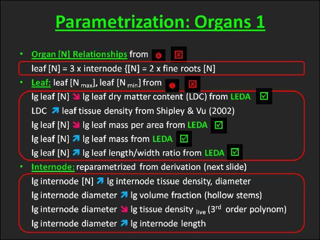
Fig. 25: Organ parametrization I

Top_________________________Next

Stem and internode paramerization

	The parametrization of stems and internodes is graphically displayed in reversed order, beginning on Figure 26 and ending on Figure 25.
	In the parametrization the stem allomety relationships determined by Niklas (1995) on 76 herbaceous species were of fundamental importance.
	Niklas (1995) did set up scaling relationships between stem diameter at ground and plant height, on the one hand, and the volume fraction of lignified tissue in the stem, on the other hand. The relationships, in principle, indicated that the stems of taller species were disproportionately more slender and lignified than those of smaller ones (compare the direction of the corresponding arrows in Figure 26).
	The third relationship of relevance to UIBM was that between lg bulk tissue density and lg diameter at ground, which was fitted by Niklas (1995) using a third order polynomial. The polynomial, in fact, tends to decrease with increasing lg diameter at ground (compare Figure 26). Since the bulk tissue density of hollow stems was measured after cutting the stem into two median longitudinal sections, the value resembles the density of living tissue and ignores empty spaces inside the stem.
	This completes the set of equations necessary to begin stem and internode parametrization in UIBM.
	The most prominent stem-related information contained in the databases is certainly the canopy height. Canopy height serves here as starting point for parameter derivation.
	Since Niklas (1995) used to fit all relationships with reduced major axis linear regression, usage of the inverse functions without reparamtrization is appropriate. Thus, the diameter at ground can be assessed from canopy height using the first relationship mentioned above. Note that serial biological reesoning had be violated here in order to make inferences about stem attributes from database information possible.
	In the next step two major simplifying assumptions are being made:
	First it is assumed that the stem can be approximated as a cone. This enables us to compute the stem volume with the formula for the cone volume: Volume = 1/3 π (diameter/2)⊃2; canopy height.
	Second, a stem is simplified to be a rod or a hollow cylinder composed of stacked internodes with each internode having identical shape. The latter part of this assumption traces back to the observation that internodes appear flat, but large in diameter at the stem base and reduce in diameter, but extend in length towards the apex. The observation I made while inspecting online images of many plant species suggested that internode volume is somewhat preserved along a stem. This rather intuitive finding entered UIBM here as simplifying assumption.
	However, the number of internodes per stem, the crucial stem attribute, that is needed to scale up/down betweeen stem and internodes, is lacking from any database. This is unfortunate, because the attribute is also necessary for scaling up/down between foliage and individual leaves, when a plant possesses only main stems. Instead, we had to rely on experimental data, which was gratefully provided by M. de Jong (unpublished). More results related to this experiment were published by de Jong (2003) in his Ph. D. thesis and his own publications cited therein.
	Still assuming that primarily nitrogen is limiting plant growth as well as plant height, the minimum canopy height is associated with the lowest internode N-concentration, and vice versa.. Niklas' (1995) first scaling relationship is applied to infer the associated diameters at ground. The associated "approximated" internode diameters are found using the first assumption made above. With those values a scaling relationship between lg internode [N] and lg internode diameter is set up.
	On the basis of serial biological reasoning we made the volume fraction of lignified tissue and the tissue density dependent on the internode diameter. Towards this end, Niklas` (1995) two other scaling relationships were reparametrized with the internode diameter replacing the stem diameter at ground. Since Arrhenatherum owns hollow stems, the density is exclusively that of living tissue and the volume fraction of lignified tissue in the internode is identical with the wall thickness of its cylindrical approximation.
	Finally, a log-log-linear relationship between the diameter and the length of an internode is set up with the canopy height and the number of internodes per stem given.

Fig. 26: Organ parametrization II

Top_________________________Next

Flower parametrization

	Procedures with respect to flower parametrization are displayed in Figure 27.
	Since pollen number is derived from seed number, I will begin with developing seed parameters.
	Seed mass and seed nitrogen concentration were simply taken from the Seed Information Database (SID) compiled at Kew Gardens. Unfortunately, however, the maximum number of seeds produced by an Arrhenatherum elatius stem was not available from the databases. At the time of parametrization the Ecological Flora of the British Isles assigned our template species merely a broad seeds per stem category (1,000-10,000). Relating the seeds weight to the maximum vegetative plant weight revealed that only a seed number at the lower margin of the category was realistic. Thus, the maximum seed number per stem was assumed to be at 1,001 and was set to that value. Hopefully, the LEDA traitbase will facilitate the provision of maximum seed numbers in the near future. Nevertheless, the seeds per stem, on the other hand, may serve as an instructive example of how important the shift from recording trait categories towards recording trait minima/maxima and medians was that LEDA accomplished.
	Technically, the pollen mass was obtained from the Palynological Database (PalDat) using the following procedure: The pollen size was measured from online pollen images available on the PalDat website. A formula for the volume of an ellipsoid was taken from Roulston, Cane & Buchanan (2000). The same authors provide also a log-linear equation that we used to calculate ln mass from ln volume.
	An Arrhenatherum-specific pollen [N] was not available from PalDat or any other database; instead we entered the average value given by PalDat for the Poaceae family.
	Finally, the maximum number of pollen per stem was received by multiplying the pollen-ovule ratio contained in the BIOLFLOR database and the maximum seed number per stem. By this means we arrived at a value of 37.161.124 pollen per stem.
	The rules that govern pollen and seed production in UIBM follow a model analysis conducted by Zhang & Jiang (2002) and further elaborated in Harder, Charles & Barrett (2006). In their evolutionary stable strategy model perrennial herbaceous plants beyond a certain environmentally determined size threshold should allocate a constant amount of resources to male function as well as to post-breeding survival and should merely vary allocation to female function in this case. In contrast, plants smaller than that size threshold were expected by the authors to be either nonreproductive or functionally male only.
	We adopted the behavior described by Zhang & Jiang (2002) using strict serial processing of pollen and seed production. In the hermaphroditic case the male function is satisfied first until the maximum number of pollen per stem is reached, and only if that threshold is passed the state of the ramet is switched to seed production.
	Notably, experimental data of de Jong (2003) suggested that Arrhenatherum reaches flowering even at the smallest canopy height.
	Arbitrarily, we let plants that grow to minimum canopy height enter generative reproduction state with the top internode having flower meristems, but do not let them begin pollen production. Unlike, plants growing with maximum nitrogen resources to maximum dry mass produce maximum numbers of both,pollen and seeds, with both sexual functions occupying identical weight.
	Although phenotypic variation in seed size is widespread among plants, seed size is known to be one of the least variable plant traits (Fenner & Thompson 2005). Reflecting this knowledge, variation in seed mass or seed nitrogen is ignored in UIBM as yet.

Top_________________________Next

Clonal growth organ parametrization

	Clonal growth organs or - abbreviated - CGOs are responsible for vegetative reproduction and play an important role for grassland species enabling them to regrow after mowing or grazing by remobilizing their carbon storage. According to the Clonal Plants Database CGOs come in 17 types, which differ largely in phenotype, location on the plant and organ origin. As CLOPLA states Arrhenatherum owns a CGO type 10, i.e. a hypogeogeneous stem (rhizome). In fact, rhizomes, albeit of epi- or hypogeogeneous type, appear to be the most common CGO type in grasslands.
	The Lateral spread in [m/yr] and the No. offspring in [shoots/ parent shoot/ year] were the two traits taken from CLOPLA and being included in the inference of CGO traits. Since the database merely records categories for the traits in question, category averages were assigned to our template species.
	In principle, the following argumentation was applied: Arrhenatherum reaches an average canopy height of 1 m. Canopies growing to this size are supposed to be subject to a twice annual mowing regime. and, hence, the plant stems grow 2 meters per year. Since the lateral spread category average for Arrhenatherum is 0.13m, we partition a constant fraction of the resources aimed at the stem to the CGO, namely 6.5%. This argumentation was influenced to a large extent by the organ origin of CGO type 10. For the same reasons, all CGO traits other than the CGO length are assigned values, which resemble those of the internode, that is produced as part of the same organ set.
	However, when the CGO length attains multiples of lateral spread / no. of offsprings rounded to the next integer the parent ramet vegetatively produces a daughter ramet.
	Overall, this represents a rather simplistic CGO parametrization. Possible improvements already claimed in Figure 27 are dealt with in the discussion.

Top_________________________Next

Roots parametrization

	In the introduction to their volume on root methods Smit et al. list key root system parameters with relevance to root functioning (Smit et al. 2000, Table 1.1, pp. 15-19).
	Table 4 replicates their list with own modifications and abbreviations. The last column indicates that all attributes referred to in the table with exception of the rooting depth are currently lacking from species trait databases.
	The lack of root-related information in the databases appeared to jeopardize the development of an individual-based model for the Central-European herb flora from the beginning on.
	The most urgently needed information was certainly the root:shoot ratio, since it allows for the computation of the final dry mass attained by the vegetative ramet. For the template species R:S-ratios and their dependence on nitrogen availability could be obtained from comprehensive experimental data of de Jong (2003).
	Nonetheless, the question of how to deal with the rest of the herbaceous flora remained to be addressed. Hence, considerable efforts were made to invent a suitable general methodology for the retrieval of species-specific root traits.
	The method outlined in the subsequent paragraph enabled us to derive dimensions of the Arrhenatherum rooting system for now, but besides that experimentation suggested that most of the parameters with functional relevance listed in Table 4 could possibly be obtained using the outlined method.
	However, because we focused on aboveground processes first during UIBM development, rooting systems were left non-functional until now and do not take up nitrogen, though. Nonetheless, the user is able to vary the nitrogen input to ramets by manually adjusting the parameter "C:N-ratio in the resources".

Table 4: Key structural root parameters

Root attribute scale	Root attribute	Functioning	Present in species-specificrait databases
Rooting system	Root:shoot ratio, based on dry mass [g/g]	Balancing above-/belowground resources acquisition	No
Rooting system	Total root dry mass [g]	Total investment of assimilates in belowground resources acquisition	No
Rooting system	Total root length [m]	Potential for nutrient or water absorption from soil.Reference for root associated microbial functioning.	No
Rooting system	Rooting depth [m]	Estimation of soil resources available for exploitation	Yes
Rooting system	Root system diameter [m]	Estimation of soil resources available for exploitation	No
Rooting system	Rooting volume [m³]	Estimation of soil resources available for exploitation	No
Rooting system	Root length density [cm/cm³]	Assessment of soil exploitation limitation	No
Individual root	Root diameter [mm]	Enables computation of root surface area	No
Individual root	Root surface area [cm²]	Determines uptake capacity for water or nutrients	No
Individual root	Root dry weight : fresh weight ratio [g/g]	Enables computation of root tissue density	No
Individual root	Root tissue density, dry mass/ volume [g/cm³]	Correlates with root longevity	No
Individual root	Specific root length, SRL [m/g]		No

Method for species-specific root traits retrieval

	Development of plant trait databases was founded to a large extent in the the collection of specimen, the despription of species and their systematic naming/classification carried out during the 17th, 18th and 19th century.
	Being aware of this, I sought to find out whether a similar pioneering and mostly descriptive phase existed in root science. And there was indeed a time period in which root scientists unburried entire rooting systems of individual species from their natural environment and made drawings of the systems with the original dimensions and the exact 3d-location of each root converted to two dimensions on paper. Results of this kind of admirable and laborious work, i.e. images of rooting systems for thousands of plant species drawn by the authors, can be found in the encyclopedicroot atlas volumes published by Lore Kutschera, Erwin Lichtenberger and Monika Sobotik (Kutschera 1960, Kutschera, Lichtenberger & Sobotik 1982, Kutschera & Lichtenberger 1992).
	I have written a computer program for root parameter extraction from digital images of scanned rooting systems using the DIPimage toolbox integrated in MATLAB. By this means we were able to assess the diameter to depth ratio for the Arrhenatherum elatius rooting system after scanning the image from Kutschera, Lichtenberger & Sobotik (1982). Along with the maximum shoot dry mass, the R:S-ratio, root system dimensions and rooting depth being assessed and assuming that root tissue density is similar to leaf tissue density (Wahl & Ryser 2000, Craine et al. 2001, Tjoelker et al. 2005) we arrived at a first guess of a possible dry mass per rooting volume that allowed us to dynamically adjust the size of the cylindrical rooting volume for the template species.
	Further experimentation with the general purpose DIPimage processing tooolbox revealed that information about total root length and average root diameter could also be gained from the images. The absorbing root surface area could be assessed by multiplying the total root length and the average root diameter given that grasses possess merely fine roots and that root hairs cover long lengths of the root epidermis (Gibson 2009).
	In other cases, coarse roots and fine roots could be separated according to their diameter.
	Since the images include drawings of the shoots to which the rooting system belongs, there is also a good chance to retrieve species-specific root:shoot ratios from the images using the UIBM organ parametrization scheme described above. The combination of shoot drawing and the wealth of additional information provided in the root atlas, such as excavation location and time of the year, plant height, plant ontogenetic stage, accompanying plant community and the detailed soil profile, may allow for a categorization of the "snapshot" that was taken on the rooting system.
	As a brief scan of root science literature indicated, more researchers had adopted the methods outlined in the root atlas volumes and they had displayed images in their publications thereby making them available for comparative studies.
	However, unfortunately certain stoichiometric and anatomical root parameters cannot be derived from the images. Among those are for example the root nitrogen concentration, the root tissue density and fine root length covered with root hairs (required for the computation of the absorbing root surface area of e.g. Dicotyledoneae).
	Nonetheless, in essence the experience with image analysis of rooting systems appeared promising enough to keep complete root parametrization for later, and to continue with parametrization of aboveground plant structure and function.
	Copyright © Jul. 2006 Dr. U. Grueters

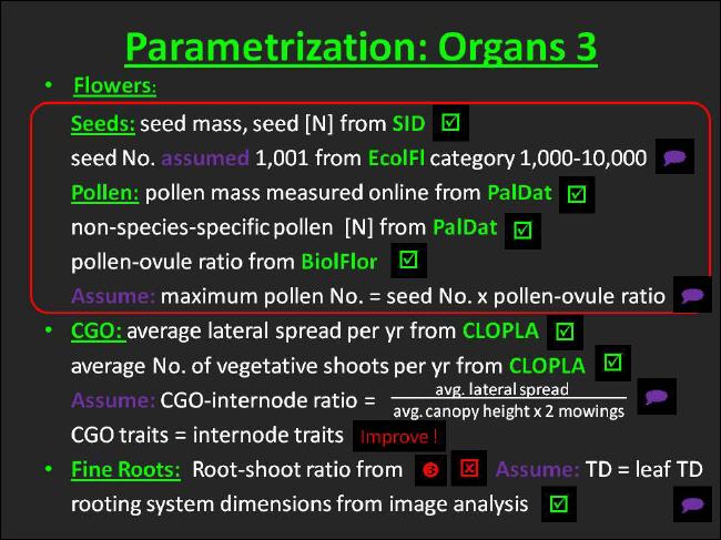
Fig. 27: Organ parametrization III

Top_________________________Next

Parametrization of partitioning

	Procedures related to partitioning are depicted in Figure 28.
	In accordance with many other ecological models UIBM's partitioning aabove- and belowground is based on measured root:shoot ratios. The Arrhenatherum elatius R:S-ratios assessed by de Jong (2003) were in qualitative agreement with the balanced growth hypothesis of Shipley & Meziane (2002): de Jong found that plants allocated preferentially more biomass to roots in his low N treatment.
	From those measurements we are able to infer root:shoot ratios for the minimum/maximum nitrogen conditions in the Central-European distribution area of the template species by using simple linear interpolation/extrapolation.
	This puts us in the position to evaluate the allocation to the varius organs contained in an organ set at low and high N as well as the C:N-ratio in the resources that are needed to build those organ sets, respectively.
	The C:N-ratio in the resources then becomes the main factor driving the partitioning. By this means partitioning is traced back to the root cause of the balanced-growth hypothesis (Shipley & Meziane 2002): that plants tend to compensate reduced capture of the limiting external resource by adjustment of their root:shoot ratio - a response, which definitely falls behind full compensation and "optimal partitioning" (compare McConnaughay & Coleman 1999).
	In UIBM linear interpolation, however, is used in general to calculate partitioning parameters, when resources C:N is not at the lower or at the upper margin.
	Assuming an invariant species-specific carbon fraction in the dry mass we begin partitioning with a routine to allocate carbon aboveground/belowground according to the linearly interpolated root:shoot ratio for the given resources C:N.
	In case a species contains coarse roots and the coarse root:fine root ratio at low/high N is known for the species under construction, belowground carbon might be further partitioned into fine and coarse root fractions once again linearly dependent on the C:N ratio of the resources. For Arrhenatherum this was not necessary, since this species is known to possess merely fine roots (see above). However, coarse root:fine root partitioning has been implemented in UIBM to preserve the universal nature of the model.
	In contrast, the linearly interpolated internode:leaves ratio allows for further partitioning of aboveground carbon. The concurrency of reaching sufficient carbon to produce an internode and to produce leaves might be used as a criterion to test the validity of linearly interpolating internode:leaves ratio. Eventually we will learn from the model, refine it and replace the linear interpolation by either a scaling relationship or any other empirical function that better fulfills the criterion.
	A constant fraction of the internode carbon held in the parameter CGO:internode ratio is finally diverted to the clonal growth organ (see above).
	The subsequent procedures accomplish the partitioning of nitrogen: The current N amount in the resources is set into relation to the sum of carbon amounts partitioned to the organs each multiplied by the maximum N concentration of that organ. This value does represent a universal factor for that species to reduce N concentrations in the organs.
	In principle, the within-organ-set allocation remains unchanged for the entire vegetative ontogenetic phase of the ramet. The underlying assumption here is that of an isometric root:shoot relationship with a slope of unity in the log/log-linear R vs. S plot.
	Nonetheless, the allocation scheme is different for the first organ set being built by a seedling. Since it contains only cotyledon(s) and roots, but lacks internode and CGO, minimum and maximum resources C:N ratios for its formation are different as well as some organ ratios.
	The allocation scheme alters also when a ramet enters the generative reproduction stage. Here the organ set is simply assumed to lack leaves - once again leading to minimum/maximum C:N-ratios in the resurces being distinct from those of the vegetative phase.
	Furthermore, we suppose that a ramet stops growing vegetative organs when it starts flowering (determinate growth). At the ramet network or - in other words - at the whole plant level this would lead to an abrupt shift of the slope in the log/log-linear plot of total shoot DM vs. total root DM, which would disappear, when logarithms of merely vegetative organ dry masses are plotted against each other.
	To conclude, in the biodiversity model proposed here the overall retreat to linear assumptions plays a pivotal role. This approach has often been chosen by ecological models facing lack of information. Here it is a response to the scarcity of partitioning information at the level of individual species.

Top_________________________Next

Parametrization of ramet growth

	The procedures described in this paragraph are graphically displayed in Figure 28.
	Plant function emanates from plant structure, which in turn mirrors the history of previous plant function. Since plant growth in UIBM proceeds in a discrete fashion, we face a period in ontogeny, when no structure is available to drive basic physiological functions, i.e. after the seed has germinated and before the ramet produces its first organ set. For that period we were in need of an alternative mechanism to drive plant growth. The same mechanism was chosen to accomplish the processing of plant growth during the early phase of UIBM development - during the time we focused on implementing the build-up of plant structure and had not yet implemented the functional basis.
	My fascination with West, Brown & Enquist's seek for general patterns in nature directed me towards using a universal scaling law as mechanism. West, Brown & Enquist (2001) provide the following general equation (their eq. 4) for ontogenetic growth:

	It is possible to insert plant traits mostly contained in databases into variables of a discretized version of equation 3 and achieve a species-specifically parametrized plant/ramet growth function:
	The seedling growth rate (SGR) is the first trait, that is needed to accomplish this. Hendry & Grime (1993) describe the methodology to measure the relative growth rate (RGR) of seedllings under optimal conditions and extrapolate the (maximum) RGR towards the seed mass to give the SGR. Seedling growth rates determined with this method for large numbers of species were originally published in database form in the Electronic Comparative Plant Ecology by Hodgson et al. (1995), but were later integrated in the Ecological Flora of the British Isles. The Arrhenatherum elatius SGR taken from these sources is then multiplied with the species-specific seed mass to compute the absolute growth rate per day of a seed.
	In consequence, we equate the current body mass in equation 3 with the seed mass, Δm with the absolute growth rate and Δt with one day, respectively.
	The seed mass, in fact, represents the second plant trait required to parametrize the species-specific plant/ramet growth function. Once again, this trait was taken from the Seed Information Database.
	The third needed variable is the maximum body mass. This variable is readily available from the completed organ parametrization for both, the minimum and maximum nitrogen supply, respectively.
	However, after transposing equation 3 and solving for the last unknown, i.e. the growth coefficient a, we finally arrive at the intended ramet growth function parametrized for the template species under the lowest and highest nitrogen supply the species pertains in its Central-European distribution area.
	In principle, the procedure implies that plants initially grow with maximum stage-dependent rate irrespective of the nitrogen being applied before they diverge and approach the N-dependent final dry mass. Since the seed N-concentration is usually higher than that of vegetative organs and since soil N-concentrations are often highest at ground level, we suppose maximum N behavior for the period shortly after germination.

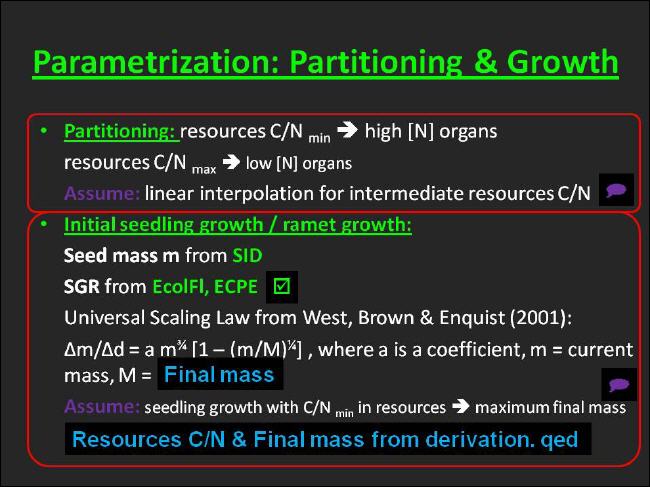
Fig. 28: Parametrization of growth and partitioning

Top_________________________Next

Parametrization of branching

	Procedures related to branching are depicted in Figure 29.
	In UIBM branching is realized in the most general way conceivable by us. Implementation of branching requires management of object location and orientation in 3d. Thus, related UIBM principles are elucidated here briefly.
	Basically, all objects displayed in the three-dimensional space of UIBM's virtual vegetation survey plot are bilateral-symmetric and have a front and a rear end, top and bottom as well as a right- and left-hand side. With the methods located in the Navigation class objects can be navigated in 3d-space just like you would navigate aircrafts. Objects might move forward or backward, pitch up or down, turn left or right and roll clock- or counter-clockwise around their front/rear end axis, respectively.
	Initially, i.e. in the seedling stage, the plant is oriented upward with its front end pointing exactly upright. Three parameters define the orientation of the seedling components: The number of cotyledons (either 1 or 2 in case the species is mono- or dicotyledoneous), the angle by which the insertion of the cotyledon deviates from the main (vertical) axis, the initial angle and the incremental angle of the cotyledon(s). To give an explanation to the workings of the latter angles: When the initial angle is 0°, the first cotyledon inserts at the "back" of the plant. With an incremental angle of 180° the second cotyledon would insert opposite to the first pointing away from the "bottom" of the plant.
	In principle, branching may commence, when a plant leaves the seedling phase. Thus, a phytomer concept is underlying the build-up of the modular plant structure aboveground during the vegetative and generative phase. In the object-oriented program a class for the construction of a composite object, named InternodeWithMeris, resembles the torso of a phytomer.
	It contains the primary meristem, which is located in central position at the end of the preceding internode and is responsible for the extension of the stem/culm by forming another internode (internode meristem) or a flower (flower meristem with determinate growth).
	Besides that, the InternodeWithMeris holds a number of leaf meristems. Those meristems are located at the surface of the internode with corresponding off-axis, initial and incremental angles defining their orientation at the insertion points.
	The activation behavior of the meristems, however, differs whether the species owns continuous or terminal leaves. The template species Arrhenatherum elatius - as most Poacean species - contains continuous leaves. In contrast to terminal leaves, whose meristem is located at the utmost end of the leaf and gets absorbed during leaf growth, the meristem of continuous leaves is positioned at the base of the leaf blade and is thus able to get reactivated, when the leaf blade is removed. The implementation of continuous leaf meristems in UIBM mimics this behavior.
	The third kind of meristems held by the InternodeWithMeris is the additional meristem. Like leaf meristems additional meristems are located at the surface of an internode (in the axils of leaves) and their orientation is given by a similar parameter set as that described above for leaf meristems. Additional meristems might be of internode or flower type. In case a species does contain only additional flower meristems, its growth is non-determinate.
	Grass species to which our template species also belongs, have a special kind of additional internode meristem: The so-called intercalary meristem, which becomes activated only after removal of ensuing internodes. Intercalary meristems enable a ramet to regrow after mowing or grazing events took place. The UIBM implementation mimics this behavior.
	The insertion points of leaves or of internodes of lower branching order that emerge from additional meristems are displaced on consecutive internodes. We named the angle, by which an internode displaces its lateral organs in comparison with its predecessor, the "divergence angle".
	Essentially, all numbers and angles necessary for the construction of the template species were estimated from drawings available as online images. The advantage of using such images is that drawers have usually made considerable efforts to draw the general appearance of that species. Since we assume that his kind of drawings is available for the majority of Central-European species, we consider this a first-class source of information.
	However, inspecting numbers of dicotyledoneous species drawings revealed also that organ size tends to decline with increasing branching order, but that organ dimensions are likely to remain unchanged. The phenomenon underlying the first observation is commonly referred to as "apical dominance" in botany.
	A likely named parameter was introduced into UIBM to simulate this behavior. The apical dominance parameter ranging between 0 and 1 is regulating a subordinate carbon partitioning step. In the example given in Figure 29 the parameter was set to 0.5. With two additional internode meristems (in the example) the internode of the main stem or, say, the internode of higher branching order receives 50% of the carbon partitioned to internodes, while each of the lower-branching-order internodes receives 25% of that. If internodes of still lower branching order were present, carbon partitioning would go on as outlined before.
	However, in accordance with the second observation referred to above internode diameter and length are reduced with their ratio held constant. In all other respects, including nitrogen concentration and tissue density, simultaneously produced internodes are identical.
	Two additional parameters allow for regulation of branching dynamics: First, there is a time for additional internode meristems to activate and, second, additional meristems hold on an activation probability. For Arrhenatherum apical dominance was set to 1, an activation probability of 0 was chosen and the activation time was turned off by specifying it to an unreasonable high value. Doing this allowed us to simulate the behavior of the intercalary meristem, which is specific to Poaceae.
	In principle, leaves experience the same treatment as internodes. Nonetheless, Arrhenatherum makes usage of these procedures merely in one situation - after a leaf has been removed carbon is partitioned to the terminal and the regrowing leaf. Since they are of the same branching order, both end up with half of the normal size.
	I shall make clear that assuming apical dominance exerts its influence merely on carbon partitioning violates the presumption made earlier that most organ attributes are dependent directly or indirectly on the inherent nitrogen concentration. Therefore, I consider the current approach to simulate apical dominance to be preliminary. Moreover, I suppose that refinement of the approach taking into account an influence of apical dominance on nitrogen partitioning is needed.
	Finally, I would like to point out that UIBM generally assumes the existence of synchronized organ growth.

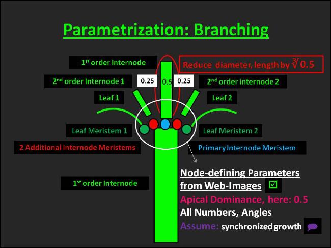
Fig. 29: Parametrization of branching

Top_________________________Next

Parametrization of plant function

Parametrization of organ function

	Procedures related to organ function are depicted in Figure 30.
	When it comes to modeling the response of vegetation to climate change, a mechanistic biodiversity model, one that is based on simulated physiological processes, has important advantages.
	Requirements concerning experimental data might be substantially lower than those of empirical approaches. For this to become true, physiological submodels, which have found widespread usage and whose parameters are known for large numbers of species or are easy to determine for others, should be chosen. Moreover, preference ought to be given to submodels,that mechanistically simulate the effects of individual climate change factors on physiological processes.
	However, in contrast to life history traitbases, which have become available in numbers on the web, development of databases with species-specific physiological traits and their publication online is in its infancy. Consequently, physiological information is rather spread out over many sources and retrieval of such information from the literature is cumbersome, though. Certainly, this is the main disadvantage of relying on physiological model components.
	Several factors might have contributed to the slow advancement of physiological traitbases: Many ecosystem models assume a uniformity of plant physiology. In accordance, the opinion that plant species show a uniform physiological behavior seems to be rather widespread among ecologists. Other ecosystem models focus on parameter heterogeneity of Plant Functional Types only, but neglect species heterogeneity. And finally, due to the absence of tradition the development of a physiological database does represent an enormous challenge. Even addressing the question of which processes and which parameters to include in such a physiological traitbase is a non-trivial task, let alone the parameter retrieval for whole floras.
	Nonetheless, weighing pros and cons lead us to provide UIBM with a functional basis. In this context, the template species Arrhenatherum elatius served us to gain experience with the retrieval of physiological parameters and test their availability.
	We decided to include a minimum set of three (mostly aboveground) physiological processes in UIBM: organ mass- and energy-exchange, organ lifespan, and processes associated with carbon/nitrogen storage.

Top_________________________Next

Mass- and energy exchange parametrization

	Among the aboveground organs leaves and internodes are considered in UIBM to contribute to the mass- and energy exchange of the canopy. Both kinds of organs are assumed to engage in photosynthesis and respiration. In contrast, fine roots and the clonal growth organ, both residing belowground, are considered to act as mass exchange organs only. As all other organs mentioned above they engage in dark respiration.
	In simulation models autotrophic respiration has traditionally been divided into two distinct components, associated either with maintaining existing structural biomass or with growing new structural biomass.
	In UIBM, however, only maintenance respiration is included as far as possible, whereas growth respiration is entirely ignored.
	This is due to the discrete nature of how growth is implemented in UIBM. A new organ set is immediately produced in a full-grown state, when sufficient carbon has accumulated. In essence, this means growing organs are not at all functionally active; they neither pursue photosynthesis nor maintenance or growth respiration during growth.
	It is assumed, though, that the amount of carbon exchanged by an organ set during the growing phase is negligible when compared with that exchanged over the rest of its lifespan. The consequence of this treatment, however, is that photosynthetic carbon gains of a growing organ set compensate for its respiratory losses.

Top_________________________Next

Leaf parametrization

	The leaf mass- and energy exchange module implemented in UIBM is based on a simulation model published by Kim & Lieth (2003).
	At first glance, this coupled model appeared to meet our needs very well:
	It constitutes of the mechanistic Farquhar, v. Caemmerer & Berry leaf photosynthesis model, which since its first publication in 1980 (Farquhar, v. Caemmerer & Berry1980) has become by far the most widely used model of this kind worldwide. Founded in detailed analysis of leaf biochemistry Farquhar and others proposed modeling photosynthesis as being limited by one of three partial processes - by the RuBisCO carboxylation rate, by the electron transport rate available for the regeneration of the primary CO2-acceptor RuBP or by the rate at which triose-phosphate is utilized for the transport of sucrose away from leaf cells (Farquhar, v. Caemmerer & Berry 1980, Sharkey 1985, v. Caemmerer 2000, Kim & Lieth (2003).
	All three photosynthetic processes are assumed to be dependent on leaf age, and all three are implied to hold an optimum dependence on leaf temperature given by an Arrhenius equation. With the corresponding small set of parameters (Vcmax = maximum carboxylation rate, Jmax = potential electron transport rate , Pu = potential triose phosphate utilization rate) and their dependencies on age and temperature of the leaf the model is quite simple, easy to parametrize from photosynthetic CO2-response curves or from measured gas-exchange data, and its application has proven to be very useful, though. The wide usage of the model suggested that parameters are available for large numbers of species, in particular for grassland species from the parametrization work of Wohlfahrt et al. (Wohlfahrt et al. 1998, Wohlfahrt et al. (1999). Moreover, Kim & Lieth (2003) took into account the maintenance respiration of the leaf to allow for model validation based on measured net photosynthetic rates. As with photosynthetic parameters maintenance respiration has been made dependent on leaf temperature using an Arrhenius equation.
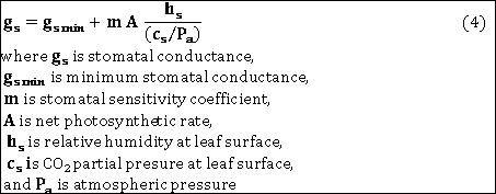
	Kim & Lieth (2003) further used the Ball, Woodrow & Berry (1987) stomatal conductance model, which has been specifically developed to work in combination with the Farquhar, v. Caemmerer & Berry photosynthesis model. The BWB model supposes stomatal conductance gs to follow the simple linear relationship:

	Kim & Lieth's third component is a general leaf energy balance model, which they adopted from Campbell & Norman (1998). It provides the leaf temperature as a function of air temperature, absorbed short-/long-wave solar radiation, boundary layer conductance, stomatal conductance and relative humidity.
	Apparently, the three model components are highly interdependent: The leaf energy balance determines the organ temperature. Organ temperature, in turn, is affected by leaf transpiration, which is partially under stomatal control. Net photosynthesis depends on leaf temperature, but also affects stomatal conductance.
	In general, those interdependencies are solved in the program with a nested iterative procedure using the Newton-Raphson method. The iteration starts with intercellular CO2-concentration set to be 0.7 times the ambient CO2 level and leaf temperature set equal to air temperature. The iteration stops when intercellular CO2 and leaf temperature do not change by more than 0.001. It is assumed that convergence has been reached in this case.
	However, whether a rebuild of the model from the description given in the paper is possible could not be taken for granted. So, that had to be tested. Thus, already in spring 2005, I wrote a prototype of the module in NetLogo following the instructions given by Kim & Lieth (2003). The prototyping experience revealed two things - first, that a rebuild in principle was possible and, second, that modifications/extensions needed to be made to the original model.
	The following modifications/extensions were applied to the UIBM module:
	(1) Since the effect of leaf ageing on photosynthesis traces back to the concomttant decline of leaf nitrogen concentration, we replaced the age dependence of the partial photosynthetic processes with more "mechanistic" linear leaf [N] dependencies.
	(2) The Arrhenius equation describing the temperature dependence of leaf dark respiration was replaced by a Q10 equation having identical shape. The Q10 equation is considered to be more common and was more consistent with how other organs are treated. A leaf [N] dependence which was lacking from Kim & Lieth's model was added in UIBM.
	(3) Stomata are known to respond to soil drying with closure. In contrast to the classical Jarvis stomata model (compare Grüters et al. 1995), the BWB model in its original form did lack a representation of this behaviour. I found this unacceptable and introduced this stomatal behaviour to the BWB model building on the formulation given by Campbell (1985):

	According to the formula the stomatal response to soil drying is mediated by leaf water potential and takes place when the water potential in the leaf falls below a critical value. In order to account for water stress in the BWB model, however, we used the multiplicator of equation 5 to adjust the stomatal sensitivity coefficient.
	(4) Kim & Lieth (2003) fitted their model to gas-exchange data measured inside cuvettes and customized their leaf energy balance equation accordingly. Hence, we had to replace it with an equation qualifying for conditions in the ambient.
	After we had completed UIBM's structural basis, we recoded the NetLogo prototype with the described modifications/extensions in Java and made it part to UIBM. With parametrizing the leaf mass- and energy exchange we gained the following experience: Although there exist several grassland ecosystem models having a leaf photosynthesis basis, such as the Hurley Pasture Model (Thornley 1988) and the REGÖK model (Fuhrer et al. 1997) and although substantial parametrization work on grassland species has been done (Wohlfahrt et al. 1998, Wohlfahrt et al. 1999), it was not possible to obtain a set of Farquhar, v. Caemmerer & Berry (1980) model parameters from the literature specifically for our template species. This was in contrast to our expectations. Consequently, we merely compared the maximum net photosynthesis results of the Kim & Lieth (2003) model with published Amax values for Arrhenatherum (Murchie & Horton 1997). Since good agreement was found, we retained the set of parameters given in the Kim & Lieth (2003) paper for Arrhenatherum elatius. The parameters describing the N-dependence of the photosynthetic partial processes and dark respiration were taken from the WIMOVAC model (WIMOVAC, Leaf gas exchange module) - assuming a uniform non-species-specific behaviour.
	Fortunately, species-specific information both, from trait databases and from the literature, were more readily available for parametrizing the BWB stomatal conductance model. In principle, for paramtrizing species with amphistomateous leaves, such as Arrhenatherum, we need maximum and minimum stomatal conductances for both leaf surfaces. In the following an outline of the procedures that we used shall be given. Morrison (1998) provide a value for the maximum stomatal conductance of Arrhenatherum elatius, i.e. 410 ± 40 mmol/m⊃2; s (or assumed absolut maximum = 450 mmol/m⊃2; s). The Ecoflora of the British Isles then has stomatal densities for both leaf surfaces of Arrhenatherum elatius, i.e. adaxial stomata density = 61 /mm⊃2; and abaxial stomata density = 13 /mm⊃2;, respectively. With those values we were able to compute maximum stomatal conductances for the ad- and abaxial surfaces. In contrast, the minimum stomatal conductance could not be derived from the literature. For that, we relied on the following considerations: Wohlfahrt et al. (1999) give a minimum stomatal conductance for the Poacean species Trisetum flavescens: 75.4 mmol/m⊃2; s. Together with ad-/abaxial stomata densities of 120 and 101 /mm⊃2; (Ecoflora) it is possible to partition the minimum stomatal conductance to give minima for both surfaces, that is adaxial: 120/221 x 75.4 = 40.94 mmol/m⊃2; s and abaxial: 101/221 x 75.4 = 34.46 mmol/m⊃2; s. Multiplying each time with the ratio of Arrhenatherum:Trisetum stomata density and assuming that dimensions of stomatal openings are equal for all Poacean species leaves us with the minimum stomatal conductances of the Arrhenatherum elatius ad-/adaxial leaf surfaces to be 74/120 x 40.94 = 25.25 mmol/m⊃2; s and 13/101 x 34.46 = 4.44 mmol/m⊃2; s, respectively. The minimum staomatal conductance is reached, when A and, therefore, A x hs / (cs Pa) is zero. The chosen stomatal sensitivity coefficients then ensure that stomata are fully open and a maximum stomatal conductance is reached, when the relative humidity at the leaf surface is 0.95, the CO2-level at the leaf surface is 800 ppm and the leaf temperature is at its optimum 25°C leading to Amax. This did complete the species-specific parametrization of the BWB model.
	The two general (not species-specific) parameters contained in the extension of the BWB model to include water stress effects on the stomatal aperture (see equation 5) were taken from Yu & Flerchinger (2008).

Top_________________________Next

Internode parametrization

	Most herbaceous species possess green stems with the capability to pursue photosynthesis - just like leaves do. Results of Hoyaux et al. (2008), for instance, illustrate the significance of stem assimilation: For winter wheat canopies they found that stem assimilation rate is equal to 63%of the leaf assimilation. With this in mind we decided to furnish not only leaves, but also internodes with the capability to exchange carbon dioxide and water. It is assumed that respective gas exchange is performed by the projected area of an internode rotated by the solar azimuth angle around its longitudinal axis during the course of a day.
	Assuming that internodes behave like leaves, all parameters of the Farquhar, v.Caemmerer & Berry leaf photosynthesis model including those related to dark respiration were assigned to the internode model.
	However, model differences ensued because internodes do not have two distinct surfaces available for exchange of mass and energy. The external surface of internodes, in fact, is treated to have pooled leaf stomatal conductance parameters. Thus, we chose a stomatal sensitivity coefficient that ensures a minimum conductance of 29.69 (25.25 + 4.44) mmol/m⊃2; s and a maximum conductance of 450 mmol/m⊃2; s is reached under the conditions descrbed in the leaf paragraph.

Top_________________________Next

Root and CGO parametrization

	Since Arrhenatherum elatius owns merely fine roots, root parametrization is limited to this kind of roots. Fine root respiration is known to supply metabolic energy not only for root maintenance. About half of the respiratory energy is directed towards the uptake of minerals from the soil. Hence, it is reasonable to assume that root respiration parameters differ from those of other organs. We suppose, that the N-dependence rather than the temperature dependence of respiration is responsible for the different behaviour.
	Unfortunately, information about root respiration parameters was lacking from trait databases.
	However, Woolhouse (1965) provides a respiration coefficient for Arrhenatherum elatius, which is apt to develop the N-dependence of root respiration. He found the respiration coefficient to be 31.5 ml O2/g Protein h at 25°C (protein was measured with the Lowry method).
	In order to convert the respiration coefficient to mg CO2/g N d, the following was required:
	mol volume at 25°C = 298.15 / 273.15 x 22.414 l = 24.465 l
	respiratory coefficient = 1 (Karlsson & Eliason 1955, Lambers & Ribas-Carbo 2005)
	molecular weight of CO2 = 44.01 g/mol
	factor to convert g Protein to g N = 1/4.3 (Conklin-Brittain et al. 1999)
	The conversion yields 5847.7 mg CO2/g N d. Since Woolhouse measured the respiration of excised root tips within hours after removal from the rest of the root, the coefficient is considered to include respiratory costs of ion uptake, but no growth-related costs. This results in a maintenance respiration coefficient of 2923.8 mg CO2/gN d and an ion uptake coefficient of the same magnitude.
	Despite its internode origin the clonal growth organ (CGO) is assumed to have the same maintenance respiration coefficient than roots do.

Top_________________________Next

Parametrization of organ aging

	In UIBM plants are modular organisms whose modules, the plant organs, undergo aging.
	Initially, aging was defined by us as a gradual (linear) decline of organ N-concentration and a concomittant descent of organ mass exchange function over the entire organ lifetime. By definition the lifespan of the organ terminates and its senescence is initiated , when the N-concentration reaches a threshold of 27.5% of the initial levels (25-30% according to Whitehead 2001). Senescence, then, is considered to lead to programmed cell death resulting in remobilization of the remaining organ [N] (Noodén 2004).
	Due to these preliminary definitions, I was out for organ lifespan information in the trait databases.
	Leaf lifespan is indeed a trait listed in the GLOPNET database (Wright et al. 2004), but unfortunately Arrhenatherum elatius was not among the 2547 species contained in the database. Instead, we relied on Arrhenatherum leaf lifespans measured by de Jong (2003). In his high N-treatment controls (50 kg N/ha a, applied as ammonium) the average leaf lifespan amounted to 45 days, whereas low N-treatment (0 kg N/ha a) shortened that to 30 days.
	At first, the result seemed surprising: Arrhenatherum was found here to be a species with the intra-species trend opposing that of the inter-species trend, i.e. that leaf lifespans of species growing at low nitrogen (N) availabilities are longer than those of species growing at higher N availabilities (Oikawa, Hikosaka & Hirose 2006). However, further inquiry revealed that de Jong's result is not uncommon: Responses of leaf lifespan to N-availability used to be inconsistent among species: Some species exhibited positive responses (like Arrhenatherum), others did show negative responses and else others were non-responsive (Oikawa, Hikosaka & Hirose 2006). The question remained how to simulate this N-dependent behaviour, but meanwhile leaf lifespan was assumed to be constant.
	Information about species-specific fine root lifespan could neither be found in the trait databases nor elsewhere in the literature. However, when fine roots were assigned longer lifespans than leaves, the population of fine roots rapidly exceeded that of leaves, root respiration rose dramatically in those model runs and soaring carbon losses finally killed the plants. Thus, in accordance with findings of Tjoelker et al. (2005) we came to the conclusion that leaf and root lifespans had to be tightly linked and assigned both the same values in the model.
	The CLOPLA database served as the primary source for the lifespan of internodes and clonal growth organ, respectively.
	In the case of internodes the senescence scheme does oppose the production scheme: While each internode is produced as a single item, senescence seizes the culm as a whole. In UIBM this behaviour is imitated by a "senescence signal" that is sent through the "objects" which comprise the culm. Either the oldest internode at the end of its lifetime or the last seeds being produced (determinate growth) might become sources of such a "senescence signal". However, according to the trait databases development rates seem to be different for generatively and vegetatively produced Arrhenatherum shoots. A shoot that has developed from a seed becomes senescent in the first year (Age of first flowering = 1 yr, LEDA Traitbase). In contrast, Arrhenatherum elatius is reported to have a (vegetative) shoot cyclicity of 2 years (CLOPLA). The shoot cyclicity as defined in CLOPLA corresponds to the lifespan of a vegetatively produced shoot in years, starting by sprouting of a bud, followed by vegetative growth, flowering and fruiting, until shoot death. Whatsoever, the chosen internode senescence mechanism will properly process both cases.
	The persistence of connection between parent and offspring ramets or - short - persistence resembles the lifespan of individual CGO-elements. For Arrhenatherum elatius a persistence of >2 years is given (CLOPLA). In a simplifying act we set the value for the CGO lifespan to 3 years, though.
	No further attempt was made to incorporate environmental effects on the lifespans of these two long-lived organs. Certainly, it would have been preferrable to get hands on the median, minimum and maximum for that trait,but given the extended lifespan of those organs it is rather unrealistic to expect that those will appear in database form in the near future.
	Nonetheless, additional model runs with the initial lifespan parametrizations revealed that the evergreen Arrhenatherum plants did not survive the wintertime with the chilling temperatures prevailing in Central-Europe. Under these conditions leaves were not able to gain sufficient carbon for the production of the ensuing organ set over their lifespan. Apparently the formulation of a temperature-dependent lifespan for metabolically active and short-lived organs is a prerequisite for the simulation of the evergreen habit. Hence, we had to address the question of how to simulate temperature-dependent lifespans. To ensure tight organ coupling preference should be given to a general description of aging/senescence - one, that is applicable to all organs and that includes the effects of organ temperature and N-concentration alike. This is what our experience with parametrizing organ lifespans suggested.
	Although approaches related to leaf economics were able to explain most patterns of leaf lifespan found in nature (Chabot & Hicks 1982, Wright et al. 2004, Oikawa, Hikosaka & Hirose 2006), we rejected to use them in UIBM because of their limited applicability to other organs.
	Instead the assumption was made that a constant fraction of the protein turned-over by the organ gets lost and that this leads to the gradual [N] decline with aging (see above). Since maintenance respiration has been frequently associated with protein turnover and is said to provide its metabolic energy primarily to this process (Amthor 2000, Lambers & Ribas-Carbó 2005, Lambers et al. 2008), we assumed further that for each carbon amount lost by maintenance respiration a constant amount of nitrogen is removed from the plant organ in question. The UIBM-implementation of maintenance respiration, in fact, is temperature-dependent, and so is now the implementation of organ aging/senescence. The Arrhenatherum parametrization, then, required us to relate the leaf lifespans measured by de Jong (2003) to the temperatures prevailing in the open-top chambers, where measurements took place.
	Tissue density appeared to be one of the N-dependent organ traits that correlated strongly with organ lifespan (e.g. Ryser 1996, Ryser & Urbas 2000 for leaf lifespan; Ryser 1996, Wahl & Ryser 2000, Eissenstat et al. 2000 for root lifespan). Tissue density has also been used in empirical models to predict organ lifespans (e.g. Moorecroft, Hurtt & Pacala 2001). The results of Walter, Rogatz & Schurr (2003) might provide a mechanistic explanation of the tissue density effects on organ lifespan using leaves as example: In their study leaves with lower N-supply developed denser tissue containing more xylem vessels with altered N-supply/-turnover capabilities.
	Following this argumentation we assumed that respective N-losses/-gains in a cm³ of tissue are proportional to the tissue density and modify the fractional N-losses in protein turnover.. We evaluated the resulting coeefficient for leaves supposing that the measured lifespans (de Jong 2003) reflect the full range of regional leaf [N] levels. An analog parametrization was carried out for roots. As already mentioned, the ingoing root lifespans were assumed to be equal to those of leaves.
	In principle, this completes the parametrization of organ lifespans. Overall, the rather qualitative model validation regarding organ lifespans described in this paragraph may serve as a good example of constructionist learning.

Top_________________________Next

Parametrization of C-/N-storage

	For sessile organisms, such as plants, reserves are an efficient and often indispensable way to withstand and overcome unfavorable environmental conditions. Virtually all plant organs take part in the storage/remobilization of carbohydrate reserves, but in UIBM the focus is laid on the ecologically important long-term carbohydrate reserves, which are located in the clonal growth organ. The remobilization of these reserves plays an important role in enabling grassland species to regrow after mowing or grazing.
	Modeling reserves in a very simplistic manner requires us to know at least the carbohydrate concentration that is commonly attained in a clonal growth organ. However, although the developers of the Clonal Plant Database have extensively studied CGO-owned carbohydrate reserves (Klimeš & Klimešová 2002), this trait is neither accessible from CLOPLA for Arrhenatherum nor for any other species.
	Nevertheless, the total non-structural carbohydrate (TNC) levels given by Klimeš & Klimešová 2002) for CGOs of various species may represent an excellent basis for estimating Arrhenatherum carbohydrate reserves (compare Tab. 5). The authors distinguish two groups of species: One group possesses (mostly belowground) rhizomes that are specialized for storage and attain relatively high TNC-levels (56.1%of the dry mass on average), whereas the other group owns rhizomes without specialization which are more often located aboveground. With 38.5% of d.m. on average the latter group did exhibit more moderate TNC-levels. Since we assume our template species belongs to the latter group, we assigned Arrhenatherum the average of the latter group.
	Due to the algorithmic rather than mathematical nature of the procedures, merely a verbal description of UIBM's C-/N-remobilization and storage routines shall be given now.
	The storage of reserves, in fact, is given high priority in the model. Essentially, this is achieved by two mechanisms:
	(1) Allowance for storage of resources is made before resources are allocated to growth (but necessarily after maintenance has been processed).
	(2) The chosen rate constant of 0.5 ensures a rapid filling rate of the reserves. The meaning of the rate constnt is: 50% of the amount missing from the maximum storable amount (38.5% of d.m.) are stored per day.
	The remobilization/storage routines are being processed by a ramet on the hour after sunrise each day. The computational interval is almost daily, though. In principle, the computation of remobilization precedes that of storage. The computation procedes as follows:
	In case the C:N-ratio in the resources is outside the range to grow a plant of regional minimum/meximum height, attempts are made to bring the ratio back to the margin of the allowable range. In the first step only local reserves are included, but thereafter remobilization is extended to reserves shared among ramets belonging to the same ramet network. If the ratio is beyond the allowable stage-dependent maximum (resources-C in excess) nitrogen is to be remobilized. If otherwise the ratio is below its minimum (resources-N in excess), carbon is sought to be remobilized. Basically, there are two situations conceivable where this might happen - (1) shortly after germination because seed [N] tends to exceed the N-concentration of vegetative tissues and (2) shortly after mowing because root function and N-uptake are not affected by this management practice.
	However, if carbon in the resources is negative after remobilization the ramet will undergo death. When remobilization turned out to be incapable to bring the C:N-ratio back to the allowable range, the substance in excess, either carbon or nitrogen, is to be stored. As above, the storage target ratio in doing this is the lower or upper boundary.
	Thereafter carbon and nitrogen are stored in proportion to the ratio to be found in the resources. This is also the default procedure as long as the c:N-ratio in the resources remains in the allowable range.
	C-/N-remobilization and storage are considered by us to be indispensable processes when grassland species are to be simulated. But overall, due the scarcity of species-specific information the UIBM implementation has been done in a very simplistic manner so far.
	This finalizes the parametrization of organ function.

Table 5: TNC-concentration in clonal growth organs

Species	TNC (%)	average TMC (%)	CGO type
Bromus erectus	about 35-40	37.5	9
Calamagrosits epigejos	about 40-50	45.0	9, 10
Phragmites australis	30-53	36.5	10 (most)
Phalaris arundinacea	41	41.0	10 (most)
Calamagrostis canadensis	up to 19		?
Calamagrosits villosa	33-51	42.0	9, 10
Carex lacustris	16-45	30.5	?
Average of rhizomatous group		38.5
Molinia arundinacea	about 50-60	55.0	10, specialized for storage
Rumex alpinus	50-64	57.0	9, specialized for storage
Polygonum bistortoides	60	60.0	9 (P. bistorta), specialized for storage
Scirpus maritimus	50-55	52.5	?, specialized for storage
Poa flabellata	up to 73		?, specialized for storage
Average of group specialized for storage		56.1

from Klimeš & Klimešová (2002): TNC = total non-sturctural carbohydrates; CGO = clonal growth organ; TNC (%) = TNC in % of dry mass; CGO-type according to CLOPLA: 9 = hypogeogenous stem , rhizome; 10 = epigeogenous stem, rhizome

Fig. 30: Parametrization of organ functions

Top_________________________Next

Outline: Closing the plant life cycle

	Life cycle is defined as the entire span in the life of an organism from one generation to the next (TutorVista.com). As described in the previous paragraphs, the life cycle in UIBM is not closed yet. The life of a ramet starts from a germinating seed and ends with seed production (certainly the ramet network lives on), but seeds are not dispersed, they do not enter the soil seed bank nor do they persist therein until conditions are suitable for new germination. The implementation of seed dispersal and the soil seed bank is not only required for closing the life cycle and sustaining a canopy over many generations in the model. it is also useful because both issues are regarded as important determinants of spatio-temporal heterogeneity, which, in turn, is a key factor regulating plant diversity (Tilman 1993).
	A wealth of information is available in the trait databases, in particular in the Ecological Flora of the British Isles, that will likely facilitate the simulation of seed dispersal and soil seed bankin a species-specific manner.
	While we already have made some progress with parametrizing the template species,implementation has not been tackled yet. However, in the following I will detail my conceptual ideas about how to simulate these processes semi-empirically and how to parametrize them from trait databases.
	The season of seed dispersal may represent a starting point. Basically, I pursue the idea to implement the season of dispersal as a switch that can be turned on or off by the user. This strategy shall allow for maximum flexibility.
	The trait is listed under the term "Time of Seed Dispersal" in the Ecological Flora of the British Isles. According to the database Arrhenatherum elatius sheds seeds in autumn (September Equinox = 22.09. to December Solstice = 21.12.). With the given season of dispersal mowing twice a year would prevent Arrhenatherum from producing any seeds, since the first cutting usually occurs in June/July with this management regime. Although very early cutting is known to prevent seed production in Arrhenatherum (Ellenberg & Strutt 2009), a total suppression of seed production with the traditional management regime does not seem reliable. Apparently, correcting the season of dispersal to include the summer (June Solstice = 21.06. to December Solstice = 21.12.) would best solve the critical issue. This is what I actually decided to do. However, Arrhenatherum does not fall into the category of species whose seeds germinate shortly after shedding. Since the persistence of Arrhenatherum elatius seeds in the seedbank is transient (less than 1 year viable) and seeds germinate in summer, we are in need of an additional mechanism that prevents the seeds from germinating in the same year. Towards this end a sufficient long time of dormancy should be introduced, though.
	Because Arrhenatherum - like most other grassland species - is an anemophilous species whose seeds are dispersed by wind, it is necessary to incorporate a wind dispersal model - one that is consistent with the conceptual framework of UIBM. PAPPUS (Takenberg 2003) is a model that simulates the flight trajectory of individual seeds as affected by wind. Although PAPPUS is consistent with the individual-based framework, it was rejected by us due to its requirement for wind fluctuation measurements. The Lagrangian dispersion model developed by Robbins (2003) fullfills better our needs. It is also individual-based, but in contrast to PAPPUS all required inputs are available from our turbulent transfer model (see below), from trait databases (seed terminal velocity, LEDA Traitbase) or from the literature (Lagrangian time scale, Robbins 2003, Poggi, Katul & Albertson 2006). Besides that, the model is simple and easy to implement/understand. However, unfortunately unlike PAPPUS this model does not take into account the effects of thermal uplifts on seed flights.
	Nonetheless, the seed position is given in Robbins' (2003) discrete-time model as follows:

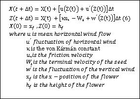
	The general assumption underlying eqs. 6 is that wind is statically neutral during seed flight.
	The first of the three equations contains the progression of the seed position in direction of the horizontal wind vector for the case that the vector is oriented exactly in x-direction. When the wind direction deviates from this, a y-component has to be included. Additionally, it is assumed that horizontal wind does not fluctuate and that wind flow is stationary in time. Hence, u'(z) is presumed to be zero.
	The second equation describes the progression of the vertical seed position.The mean uplift is given by the von Kármán constant times the friction velocity. The terminal velocity which is available from the LEDA Traitbase subtracts from the uplift. Additionally, fluctuations in the vertical wind flow are accounted for in the equation.
	In the last equation the initial conditions are defined. Essentially, seeds are considered to originate from a point source, i.e. a specific flower location.
	The mean horizontal wind flow remains as the single input for computing the horizontal seed position. As part of the turbulent transfer model being effective above and within the canopy (Campbell & Norman 1998, Teh 2006) the vertical profile of the horizontal wind is at our disposal. The computation of the wind profile itself is based on the speed and direction of the horizontal wind at a reference height above the canopy, which is an input to UIBM.
	The equation for the mean horizontal wind flow formulated by Robbins (2003) as in Campbell & Norman (1998) and Teh (2006) is:

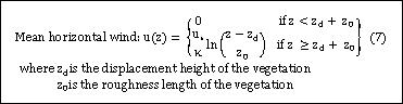
Computation of the vertical wind fluctuation requires the Lagramgian time scale as input. This parameter is likely available from Robbins (2003) or might be approximated by the Eulerian time scale as in Poggi, Katul & Albertson (2006). The respective equation is given by Robbins (2003) as follows:

	The virtual vegetation survey plot in UIBM is planned to contain periodic boundary conditions, so that seeds which leave one boundary during their flight reenter the 3d-space through the opposite boundary. Periodic boundaries will enable us to study the consequences of species turnover locally, even though the Lagrangian seed dispersal routine will allow for the computation of species-specific migration rates.
	As part of the dispersion model it is further assumed that seeds are not released from a flower until the horizontal wind speed exceeds a certain species-specific threshold. Only then the dispersal routines are activated. Basically, this approach determines the minimum radius around a flower at which seeds fall to the ground.
	Whatsoever, when a seed hits the ground it will enter the soil seed bank. Following the agent-based paradigm, the seed bank will be simulated as a grid of squares, whose dimensions might be optimized in virtual experiments.
	In principle, the fate of the seeds that have entered the seed bank via the seed rain is diverse. Losses from the seed bank occur either due to seed mortality or due to germination (Buhler 1999). Mortality, in turn, can result from physiological seed death or from biotic interactions, such as pathogenic decay or predation (Buhler 1999). Although I believe that biotic interactions are simulated best in an agent-based manner, the quantification of the related seed losses is beyond the scope of this model, at present. Unlike, physiological seed death and at least some decay is unavoidable and occurs also in seedbanks for ex-situ conservation of plant species. Hence, these losses could be taken into account with the help of the Seed Information Database (SID), which contains traits that are related to storage conditions in conservational seedbanks. SID provides a half life of 5.3 years for Arrhenatherum elatius seeds stored under open conditions in a temperate climate. From that trait a minimum daily death probability present in soils can be inferred. In principle, associated seed losses should be accounted for first.
	Using trait databases it will likewise be feasible to quantify seed losses due to germination.
	According to Kleyer (1995) half of the literature sources state that the temperature range suitable for Arrhenatherum germination lies between 2-5°C and 35°C, whereas the other half stresses that it lies between 5°C and 35-40°C with an optimum at 24-30°C. From the pooled ranges we can conclude that Arrhenatherum seeds do not germinate below 4.25°C or above 36.25°C.
	The Ecoflora of the British Isles further lists a maximum temperature at which 50% of the seeds germinate, i.e. 30°C. Thus, between 30 and 36.25°C,we would find half of the seeds germinating.
	Assuming a symmetric germination behaviour a similar range might be found at the lower end, between 4.25 and 10.5°C, respectively.
	Nonetheless, it remains to be clarified, what the germination probability is like in the range 10.5 to 30°C.
	The Seed Information Database gives a mean germination fraction of 95.17% with highest values measured in part outside the optimum range of 24-30°C mentioned above. Thus, we will not accentuate germination accross the optimum range. We rather arrive at a constant 95.17% germination fraction between 10.5 and 30°C.
	The resulting Arrhenatherum germination probabilities across a range of soil temperatures are graphically summarized in Figure 31.

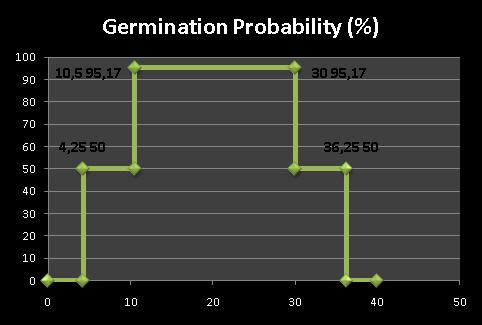
Fig. 31: Germination probability vs. temperature

	Since the above relationship has been derived from germination experiments conducted under constant climatic conditions in the laboratory, the germination probability references to an average temperature that has prevailed over the entire germination phase.
	Hence, it remains to be clarified how this relationship could be applied to the variable environmental conditions prevailing in UIBM. This is, what I want to make clear in the following.
	I intend to use a weighted averaging procedure to calculate the germination probability for a day. For instance, if the temperature in three of the hours before sunrise has stayed slightly below 10.5°C, but for the rest of the sunny day the temperature did range between 10.5 and 30°C, the calculation would yield: (3h x 50% + 21h * 95.17%)/24h = 89.52%.
	The germination probability averaged over a period that reaches back one germination phase plus a safety margin shall be used to estimate the fraction of seeds that start germinating on a day. When these seeds have completed germination, a re-computation based on the real temperatures that have prevailed during the germination phase would yield the "true" germination probability, which could eventually be used for removal of surplus seeds.
	The ECOFLORA provides another trait that might be useful for the parametrization of the seed bank, namely the maximum seed bank density that has been measured in the field (= 4792 per m⊃2; for Arrhenatherum elatius). Under the assumption that this represents an insurmountable threshold, we may stop seed dispersal entirely when the density has been attained everywhere on the plot or we may stop germination in specific square grids, where the density has reached the threshold.
	If in the end these universally applicable concepts are substantiated into implementation UIBM will be capable to embrace the life cycle of many plant species.

Top_________________________Next

Scaling up from the organ to the canopy level

	Having implemented the mass-/energy-exhange functions of individual plant organs and their dependencies on local environmental factors we are now in the position to scale those processes up to the canopy level. Certainly, each leaf modifies the environment of adjacent leaves by reducing irradiance and wind speed, and either decreasing or increassing carbon dioxide levels and vapor pressure deficit dependent on effective photosynthetic and transpiraion rates, respecively.
	The cumulative effects of organ function, however, cause the difference between within- and above-canopy microclimate to increase with increasing canopy depth. The gradient induced by organ functioning, on the other hand, is being reduced through coupling with the atmosphere.
	Traditional canopy gas exchange models developed from predecessors which modelled the canopy as a "big leaf" assuming homogeneity of within-canopy microclimate. When developers began to take into account the mutual influence of canopy structure and microclimate they solved the opposite problem, i.e. scaling-down from the canopy to the leaves, by applying a layered approach.
	In principle, we adopted similar approaches for our scaling-up issue, but because you might bre more familiar with the traditional argumentation line we start our discussion with the atmospheric environment at a reference height well above the canopy, proceed then with the wind and scalar profiles that unfold above the canopy and cease with the corresponding wihin-canopy profiles.
	An overview of UIBM's scaling-up scheme is given in Figure 32.

Atmospheric environment at reference height

	In the simplest case the input to UIBM consists of a set of analytical equations for various climate variables that are applied to a reference haight well above the canopy. This sort of equations is being used for solar radiation and temperature, respectiveley. In principle, the analytical equations simulate long-term averaged annual and diurnal fluctuations of the environmental variables.
	Solar radiation is supplied in analytical form as potential global radiation. The set of equations required for its calculation was taken from the CoupModel. The equation numbers used in the following refer to the original numbering set up in this model and are linked to the online Official Documentation of the CoupModel.
	Potential global radiation on an hourly basis is calculated with a function of the solar constant and a geometric scaling function (CoupModel eqs. 4.92, 4.93). The latter holds dependencies on the sun's position at the sky and the slope of the soil surface in N/S- and W/E-direction (CoupModel eq. 4.93).
	Calculation of the sun's position, in turn, is based on the azimuth angle, elevation angle, zenith angle and hour angle of the sun (CoupModel eqs. 4.95 - 4.101). In consequence, the entire derivation of hourly potential global radiation values is dependent on the hour of day, day of year and latitude, respectively.
	Partitioning of the global radiation into direct/diffuse photosynthetically active radiation (direct/diffuse PAR) and direct/diffuse near-infrared radiation (direct/diffuse NIR, altitude-dependent) was done following the code of the CANOAK model (Baldocchi & Harley 1995). The radiation components as calculated by the CANOAK model were compatible with inputs required by the Kim & Lieth (2003) leaf photosynthesis model. Additionally, the CANOAK results appeared more realistic to me than those of other approaches that I tested.
	An analytical description of the air temperature was also adopted from the CoupModel (CoupModel eq. 8.7). The calculation of the annual temperature cycle needs the annual mean air temperature and the amplitude of the mean as inputs. Likewise, necessary parameters for the calculation of the diurnal temperature cycle are the mean of the diurnal temperature range and the amplitude of that range, respectively. We estimated the input parameters on the basis of air temperature data of the year 2000 from the meteorological and air-quality measurement station Linden (Luftmeßstation Linden), which is located in the south-east of Giessen, Germnany (longitude: 8°41’11,5’’, latitude: 50°32’3,5’’) and is kept in operation by the Hessian State Agency for the Environment and Geology (HLUG).
	At present, the remaining environmental variables for the reference height, i.e. the partial pressure of carbon dioxide and oxygen in the air, wind direction and wind speed, atmospheric pressure and relative humidity of the air, are held constant, but are adjustable by the user.
	For the future it is planned to extend the model and allow the user also to import environmental variables for the refercne height measured at a meteorological station and run the model based on that input.

Top_________________________Next

Atmospheric environment above the canopy

	In UIBM modeling the turbulent transport of momentum, heat and mass through the constant flux layer above the canopy is based on K-theory as outlined by Campbell & Norman (1998). In K-theory the flux density of an entitiy is dependent on the underlying gradient of that entity times an entity-specific porportionality constant. In this sense, K-theory resembles the kind of equations used for moleculrar diffusion, but replaces molecular transport coefficients with turbulent counterparts. The mechanisms underlying turbulence, however, are different from those driving molecular transport. Over canopies, trubulence is driven by mecahnical action of wind moving over a rough surface and by buoyancy arising from strong upheating or cooling of the surface (Campbell & Norman 1998).
	In the logarithmic profile equations for wind (eq. 9), temperature (eq. 10), water vapour (eq. 11) and carbon dioxide (eq. 12) only mechancical forces of turbulence are taken into account. This kind of equations results from integration of respective K-theory equations from the excahnge surface at displacement height plus roughness length to height z (Campbell & Norman 1998)).
	The friction velocity contained in eq. 9 is a kind of scaling factor. In principle, it represents the rotational velocity of an eddy passing along the exchange surface at d + z_m (Campbell & Norman 1998). It can be determined by rearranging eq. 9 and solving the reusulting eq. 13 with the knowns, reference height and wind at reference height (Teh 2006).
	The zero plane displacement height has been empirically determined by many researchers to amount to 0.64 times the canopy height (eq. 14).
	According to Teh (2006) several researchers have measured the roughness length for momenutm to be 0.13 times canopy height (eq. 15a). Yang et al. (2008) give a roughness length of 11 mm over bare soil (eq. 15b).
	Campbell & Norman (1998) furher point out that the exchange of momentum within the canopy differs from the exchange of scalars, such as heat and water vapour (Garratt & Hicks 1973, cited therein). This consideration lead to eq. 16. It is assumed here that carbon dioxide is exchanged like the other scalars (compare eq. 16).
	In the future, it will be straightforward to repalace eqs. 9-12 with a set of equations (teir eqs. 7.21-7.27) that is also given by Campbell & Norman (1998), but acounts for buoyancy effects on turbulent transport.

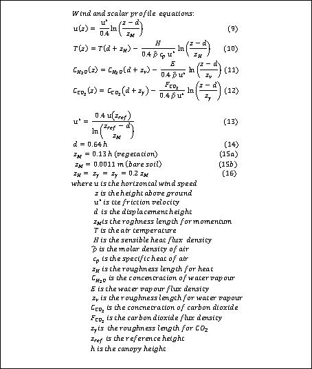
Top_________________________Next

Atmospheric environment within the canopy

	Since Arrhenatherum is commonly found in dense vegetation types, a classical layered approach was well suited for simulating the radiation interception that leads to the rapid decline of light levels with increasing canopy depth.
	A classical layered approcach was also chosen to simulate the turbulent transfer between the atmosphere and the aboveground plant organs inside the canopy. In this modeling scheme each layer below the canopy height is considered to exchange substances with adjacent layers. The canopy layer thus represents the ocal environment which plant organs exchange substances with.
	In principle, the chosen computational routines are in line with the ABM paradigm, that agents act according to their local environment.

Radiation interception model

	The radiation interception model implemented in UIBM follows the outline given by Teh (2006). In principle, the approach is based on Lambert-Beer's law, whose applicability to plant canopies has been first substantiated by Monsi & Saeki (1953, cited by Teh 2006 ( p. 70)).
	However, unlike Teh (2006) who deals with whole-canopy radiation interception in his model, we adopt his equations to radiation interception done by canopy-layers. In doing so, we ignore procedures averaging over the whole canopy and we replace whole-canopy leaf area indices with layer-specific counterparts, etc.
	The entire set of equations shown below is being applied to the photosynthetically-active (PAR) and the near-infrared (NIR) radiation component. Certainly, different parameter-sets are being used for the PAR- and the NIR-case, respectively. All irradiance components referred to in the equations might be either expressed in units of W/m⊃2; or micro mol / m⊃2; s.
	Equations 9-11 contain transmission functions for different irradiance components.
	Equation 9 covers the fraction of the direct component that is transmitted to the layer lying beneath. The canopy extinction coefficient k_dr given by Teh is based on the assumption that the orientation of intercepting plant organs is well approximated by a hemi-spherical orientation, which means that their orientation is almost random.
	Equation 10 deals with the transmitted fraction of the direct component taking into account effects of scattering. The scattering coefficient is given by Teh to range between 0 and 1. In principle, scattering leads to a reduction of the canopy extinction by squareroot alpha, though.
	Equation 11 calculates the transmitted fraction of the incident diffuse component. Eq. 11 seems to be as simple as eq. 9. However, derivation of k_df is rather complicated. Since diffuse radiation emanates from all sky directions some integration over the sky directions is required. The resulting equation does not have an analytical solution, it instead requires to be solved numerically. Finally, an empirical relationship between k_df and the leaf area index could be established (eq. 3.29 of Teh 2006).
	In the following equations we move towards the three relevant irradiance fluxes that pass through the canopy. We have to distinguish the following transmitted components: total direct irradiance including scattering (eq. 12), direct irradiance (eq. 13) and diffuse irradiance (eq.15). As a rule the term (1-p) which quantifies the negative influence of caopy reflection and the transmission functions described above enter these equations.
	Equation 14 calculates the flux of scattered irradiance as the difference between total direct and direct fluxes. The difference is cut in half, because we are concerned in the equations with leaf area indices, which do actually represent only one side of the leaf area.
	UIBM further distinguishes sunlit and shaded leaves, since this kind of canopy gas-exchange models has been shown to be superior. Thus, equations 16 and 17 calcuate sunlit and shaded leaf area indices. In UIBM the fraction of the shaded leaf area present in a canopy layer is used in the following way: A leaf area object is assigned to be shaded when a uniformly-distributed random number is below the shaded fraction, and to be sunlit otherwise. In principle, sunlit leaves are exposed to direct, scattered and diffuse irradiance, whereas shaded leaves are reached only by scattered and diffuse irradiance. In case of the direct radiation the orientation of the leaf area to the sun matters. On the basis of the direct radiation and the angle between the sunbeam vector and the surface normal the intensity of the radiation perpendicular to the leaf area is calculated. This computation is based on Lambert's cosine law.

Top_________________________Next

Turbulent tranfer model

	In contrast to the logarithmic wind profile that prevails above the caonopy the profile inside the canopy is exponential in nature. The horizontal wind speed at canopy heitght is given by eq. 9. From there it declines exponentially with canopy depth (eq. 26, from Teh 2006).
	According to Teh (2006) a similar relationship exists for the various transfer coefficients (eq. 29). It is being assumed that wihin-canopy transfer coefficients are identical for all entities (see eq. 27). Hence, all coefficients vary in similar manner with the height above ground and depend on the friction velocity (according to eq. 27). The apllication of eq. 27 to the canopy height, however, reveals maximum transfer coefficients that are valid at canopy height (eq. 28).
	Layered models have been in usage for a long time (Goudriaan 1977, Chen 1984, L'Homme 1988, L'Homme 1991). In accordance with this tradition transport of heat (eq. 30), water vapour (eq. 31) and carbon dioxide (eq. 32) within the canopy is modelled in UIBM following a layered approach given by Anda & Kocsis (2008). In the respective equations the reciprocal of the transfer coefficient of an entity divided by the layer thickness resembles the resistance to the transport of that entity through the canopy layer under consideration.
	H i, E i and F CO2,i represent fluxes which are computed by integrating over all plant organs that exhange mass and energy with layer i. When i equals 1, T a,i - 1, C H2O,i - 1 and C CO2, i - 1 are the temperature, water vapour and carbon dioxide concentration at reference height, where commonly meteorological measurements take place (Anda & Kocsis 2008).
	In UIBM we chose the layer thickness to be 15 cm. This complies with the size of the largest plant organs that exchange gases with the environment, i.e. the internodes.

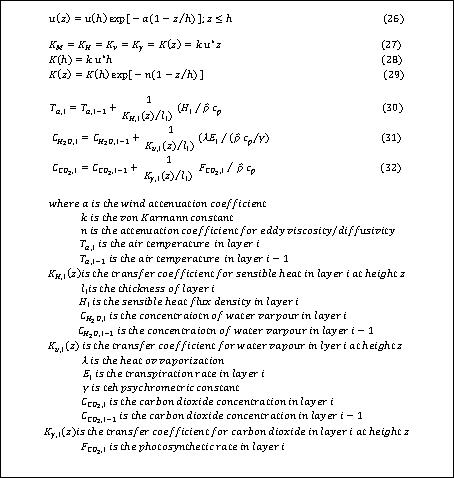
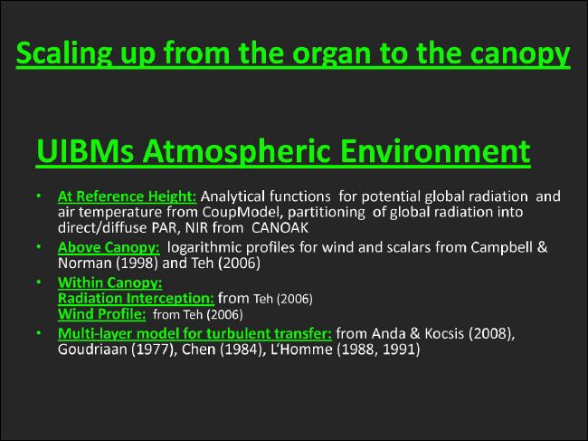
Fig. 32: Atmospheric environment employed in UIBM

Top_________________________Next

Fig. 33: Summary

Navigator

You are here: Model Parametrization -> UIBM Development -> Home

Local Navigator: Λ Top <- Previous -> Next

Sub-Page Navigator: Project Aim & Objectives <- Model Design <- Model Parametrization

Whole-Page Navigator: Home -> Background -> UIBM Development <- Virtual Experiments <- Outlook: Virtual Ecology

Print this page

The Species Construction Manual

Contents of this page

Introduction

Preconsiderations

Parametrization of plant structure

Organ parametrization

Leaf parametrization

Stem and internode paramerization

Flower parametrization

Clonal growth organ parametrization

Roots parametrization

Table 4: Key structural root parameters

Method for species-specific root traits retrieval

Parametrization of partitioning

Parametrization of ramet growth

Parametrization of branching

Parametrization of plant function

Parametrization of organ function

Mass- and energy exchange parametrization

Leaf parametrization

Internode parametrization

Root and CGO parametrization

Parametrization of organ aging

Parametrization of C-/N-storage

Table 5: TNC-concentration in clonal growth organs

Outline: Closing the plant life cycle

Scaling up from the organ to the canopy level

Atmospheric environment at reference height

Atmospheric environment above the canopy

Atmospheric environment within the canopy

Radiation interception model

Turbulent tranfer model

Navigator

Copyright © Apr. 2010 Dr. U. Grueters